Often, we would like to be able to model probability distributions of high-dimensional data points that represent an overall (much lower dimensional) concept. This lets us learn relevant characteristics of the data in question and also allows us to easily sample from our data distribution.
To understand what it means to represent something with a lower-dimensional concept, think of the difference between an internal machine’s representations of an image, and how you might describe that same image to your friend Alice.
To Alice, you might simply say “It’s a hill, with a tall tree and a horse on top”, when describing an image that takes a matrix of many millions of pixels to store on a computer. The “hill, with a tall tree and a horse on top” is a lower-dimensional representation of the image (32 bytes in ASCII), and one that only works if Alice understands how to translate these higher-level concepts into an image.
More specifically, Alice understands, based on prior experience, that there are constraints about the way images work in the world: horses generally have four legs and stand with their feet on the ground, trees are generally not purple, and typically hills only exist outside, so a sensible backdrop would be sky. Image, video, text and auditory signals contain combinatorically gigantic numbers of configurations, but most of these configurations will never exist. All of this learned context about the data distribution is what allows Alice to hear your description of the image, and imagine one that is reasonably similar, up to a point. The motivating question of this blog post is: how do we design our models to learn this kind of background context, as well as the right kind of low-dimensional representation?
Some real-world examples of these kinds of constraints are:
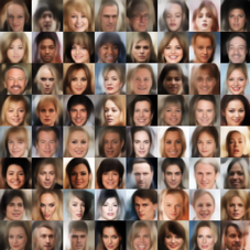
- Human faces are not going to look random. There will be some structural constants across all faces, for example, for any upright human face, the eyes will be positioned above the nostrils and the nostrils will be positioned above the mouth. Faces also exhibit certain attributes – e.g., male/female, skin color, eye color, smiling, frowning – many of which are correlated (a face with a prominent mustache is far more likely to be male than female, for example).
- Clothing: there are many different styles, colors, etc., but they must all be contoured, at least somewhat, to the human body.
- Music: There are many different styles, instruments, etc., but only a fixed number of genres and harmonious rhythms.
- Speech patterns: There are many different accents, intonations, etc., but a more or less fixed set of words and phonemes.
In this blog post, we shall examine the mechanics of VAEs, focusing particularly on the cool parts – the applications – while contemporaneously providing enough of an underlying intuition to understand how they work at the high-level. For an in-depth mathematical derivation of VAEs, we encourage the reader to check out the original VAE paper by Kingma and Welling[1].
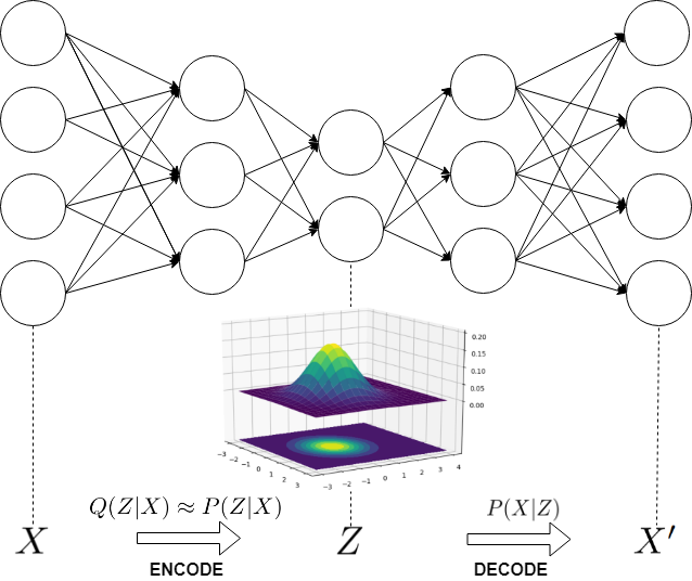
The goal of VAEs is to learn informative content about the data residing in a high-dimensional space (X) within a low dimensional latent space (Z) that describes the distribution of concepts in the data.
The main way that VAEs differ from typical autoencoders is that they constrain their internal Z distribution to be close to a fixed prior over Z, which allows for easier sampling from the model. A vanilla autoencoder learns to map X into a latent coding distribution Z, and the only constraints imposed on this are that Z contains information useful for reconstructing X through the decoder. But, what if you wanted to sample from the distribution that represented your data? How would you do it? It may be the case that your Z values are concentrated in certain regions of Z space, but, unless you were logging all of the Z values that your encoder created during the process of training, you don’t have any good way of picking an arbitrary Z value based on some criterion, and being confident that the X generated by applying the decoder to that Z will represent a valid member of your data distribution.
Sampling the Z-Space distribution
Suppose that we want to sample from our data distribution P(X). Via brute-force, this is computationally intractable for high-dimensional X. But what if we could learn a distribution of latent concepts in the data and how to map points in concept space (Z) back into the original sample space (X)? How might we go about doing so? Let us recall Bayes’ rule:
$latex P(Z|X)=\frac{P(X|Z)P(Z)}{P(X)} = \frac{P(X|Z)P(Z)}{\int_Z P(X,Z)dZ} = \frac{P(X|Z)P(Z)}{\int_Z P(X|Z)P(Z)dZ}&s=3&bg=f8f8f8$
The representation in the denominator is obtained by marginalizing over the joint distribution of X and Z. Note that the argument of the integral can be written using either the joint distribution or the product of the likelihood and prior. Unfortunately, that integral is computationally intractable for high-dimensional problems, so a stand-in must be used.
One possible solution is to sample P(Z|X) via Monte Carlo estimates. A typical Markov Chain Monte Carlo (MCMC) approach involves jumping to a new configuration in Z-space according to some acceptance criterion, given the current configuration. Notably, if we consider relative transition probability as a Metropolis-Hastings sampler does, we stochastically accept the transition to a new point in Z-space according to:
$latex P_{accept} = \frac{P(Z_{new} | X)}{P(Z_{current} | X)}&s=3&bg=f8f8f8$
Note that can avoid having to marginalize over the joint distribution, since the terms cancel in the division. Under minor assumptions and sufficient iterations, ergodicity1 in the sampling is guaranteed, allowing a random walk in Z-space according to the posterior distribution.
However, several issues emerge, including 1) time required for the walk to converge to the posterior 2) step size in Z-space, 3) separated multi-modal distributions (where multiple high-probability regions are far apart so transitions to them take a really long time), and 4) sequentially conditional dependencies in the sampling, i.e., a small step size will require several random steps to get a good sampling over Z-space.
VAEs employ a radically different approach: instead of relying on convergence of a Markov chain, we select a nicely parameterized distribution Q(Z|X), e.g., one we can parameterize with a neural network, to approximate P(Z|X) as closely as possible, under the parametric constraint. At training time a VAE learns to reconstruct samples in X using the approximation Q(Z|X), and when generating data, we sample the learnt Q(Z|X) approximation and run a feed-forward pass over the remainder of the network to generate a sample from X.
How do we compare two distributions? One way is through minimizing KL divergence:
$latex D_{KL}(Q(Z|X)||Q(Z|X))&s=3&bg=f8f8f8$
Unfortunately, we do not know P(Z|X), but it turns out that through mathematical manipulation, this becomes equivalent to maximizing what is known as the “variational lower bound”:
$latex E_Q\left[ log(p(X|Z) \right] – KL(Q(Z|X)||P(Z))&s=3&bg=f8f8f8$
Note that the expectation term (EQ) looks like a conventional MLE term, while the KL-divergence term effectively pulls the approximating distribution Q toward a prior. This prior is commonly chosen as an isotropic Gaussian (conjugate priors tend to be mathematically convenient). Note also that in the expectation, there appears to be some kind of decoding term, i.e., X given Z, while in the divergence, there appears to be some sort of encoding term, i.e., Z given X, which suggests that a good solution might take the form of an autoencoder.
While it may not be immediately obvious, we can use the variational lower bound as an optimization criterion for learning a representation that maps samples from the original input space to Z-space, where the latent vectors will be distributed as approximately Gaussian. Sampling from the Gaussian distribution in Z-space, we can construct inputs from the original data distribution. However, it would help if we had some hidden layers, to quash X to Z and reconstruct X from Z. Adding those, it starts to seem like we can maybe do some sort of backpropagation, but how do we do so while jointly tuning Q’s parameters?
The re-parameterization trick
VAEs typically select Q to be Gaussian with mean μ and covariance matrix Σ. For mathematical convenience, P(Z) is typically a zero-mean isotropic Gaussian. Observe that we can maximize the variational lower bound via stochastic gradient ascent, wherein, during the forward pass, for each value of x, we sample a value of z, according to Q, and use the results as batch updates. Unfortunately, a random sampling operation has no gradient, so we need to math-smith the layer. By separating the sampling operation from the parameters of the distribution, we can re-write sampling as a deterministic function on μ and Σ that takes X and ϵ ~ N(0,I), where z ~ z ~ Q(μ,Σ|X) is equivalent to z=μ(X)+ϵΣ-1/2 (X),ϵ ~ N(0,I). Thus, we can backpropagate gradients of loss with respect to μ and Σ, with no update to the stochastic sampling.
VAEs in practice: applications and extensions
In addition to the applications enumerated at the beginning of this blog post, VAEs can also be used for many other interesting applications including de-noising, image in-painting, image segmentation and super resolution. However, stock VAEs often need to be enhanced to accommodate a number of generative applications. This can easily be accomplished with a few refinements, for example, for many applications, we would like to be able to generate not only likely samples over a dataset, but also likely samples for a particular type of data from a dataset. When synthesizing speech, we want the network to utter particular phrases; not just a random sampling of words. We may also wish to use various accents/dialects, intonations, emphasis, etc. The same holds for other less obvious applications as well, for example, for fashion synthesis, we would like to see how a person might look in a garment, given the type of garment, the person’s body type, the person’s pose, the person’s face, etc.
To be a little more quantitative, stock VAEs allow one to generate samples from X according to P(X), but this alone allows no control over the type of samples generated. If we have some metadata, however, about the samples we want to generate, we can augment the VAE to generate only samples that follow particular metadata targets. So how do we decode from a particular section of Z-space, conditioning on metadata about the types of samples that we wish to generate? There are several ways, but one easy way to go about doing this is via conditional VAEs [3], where, given our metadata, Y, we maximize likelihood on P(X|Y) by modelling Q(Z|X,Y) and P(X|Z,Y). While conditioning a VAE may sound complicated, in practice, it amounts to concatenating a vector of metadata both to our input sample during encoding and to our latent sample during decoding. As a practical example, Lassner et al. [4] synthesized a generative model of people with various outfits, conditioned on pose and color. They employed a 3D-model for conditioning on pose and a vector of colors for the variety of colors that an outfit could assume. They used a conditional VAE to generate rough sketches, stacked with an image-to-image translation network for creating fine-grained textures.
VAEs can also be applied to data visualization, semi-supervised learning, transfer learning, and reinforcement learning [5] by disentangling latent elements, in what is known as “unsupervised factor learning”, but that is a subject for another blog post [6].
1 A random process is ergodic if its temporally averaged state is the same as its average state probability.
References
[1] D. P. Kingma and M. Welling, “Auto-encoding variational bayes,” ArXiv Prepr. ArXiv13126114, 2013.
[2] “Under the Hood of the Variational Autoencoder (in Prose and Code).” [Online]. Available: http://blog.fastforwardlabs.com/2016/08/22/under-the-hood-of-the-variational-autoencoder-in.html. [Accessed: 30-Apr-2018].
[3] D. P. Kingma, S. Mohamed, D. J. Rezende, and M. Welling, “Semi-supervised learning with deep generative models,” in Advances in Neural Information Processing Systems, 2014, pp. 3581–3589.
[4] C. Lassner, G. Pons-Moll, and P. V. Gehler, “A generative model of people in clothing,” ArXiv Prepr. ArXiv170504098, 2017.
[5] I. Higgins et al., “Darla: Improving zero-shot transfer in reinforcement learning,” ArXiv Prepr. ArXiv170708475, 2017.
[6] C. M. Wild, “What a Disentangled Net We Weave: Representation Learning in VAEs (Pt. 1),” Towards Data Science, 15-Apr-2018. [Online]. Available: https://towardsdatascience.com/what-a-disentangled-net-we-weave-representation-learning-in-vaes-pt-1-9e5dbc205bd1. [Accessed: 08-Jun-2018].
Leave a Reply